During this semester, you will use the Pasco 850 Universal interface
connected to a computer and several software packages to collect and analyze
data and present your results. Most of the time, when doing experiments,
you will work as a team of two. Each team will have one Pasco 850
interface and a laptop computer to work with. All students are required to
participate in all activities and stay until the session is dismissed.
Laboratory exercises are not just about
getting the right result, but about recognizing that fundamental physics
principles shape our everyday experiences and underlie many of the devices that
we use in our personal and professional lives. Please do not treat the
laboratories as cookbook exercises. Permit yourself to think! Thoughtful answers to the questions
in blue will give you most of the laboratory credit.
Open a Microsoft Word document to keep a live journal of
your experimental procedures and your results. Include all deliverables,
(data, graphs, analysis, outcome). Write a 'mini-reflection' immediately
after finishing each investigation, experiment or activity, while the logic is
fresh in your mind.
What 'Deliverables' mean in a physics lab report
In a physics lab course, deliverables are the specific items you must
submit to demonstrate what you did, what you measured, and what you learned.
They are the products of the lab activity.
Grading scheme for all labs:
25% for completion
In order to receive full
credit, you have to complete the entire lab and answer all parts.
Use full sentences explaining your results, show your work, insert and properly label tables
and plots, proofread, and use correct units. Make comments if you are
stuck or if your results seem to have errors. Mention what could have
caused these errors in your results and how the results could be improved. The journal
will help
you think about the material.
25% for accuracy
You do have to put effort into
these labs. This is a 4 credit-hour course with lab, so, just like for
in-person labs, you have to set aside time to work on the labs.
50% for the mini reflections and a short summary
reflection at the end of your journal, i.e. a
personal account of your experience with the lab. It should be written
in the first person. You can format it as a report to a friend or
acquaintance.
You should reflect on the material and mention how well you understood
it.
Did you understand what you were doing during an exercise or activity, or did
you just follow instructions? Do your results make sense to you, or do you expect them to be wrong? Why? Do you have suggestions on how to improve the exercise or activities so students
can learn more from them? ...
Some of the phrases you may want to use are:
The most important thing was...
I learned that...
At the time I felt...
This was likely due to...
After thinking about it...
Later I realized...
This was because...
This was like...
I wonder what would happen if...
I'm still unsure about...
...
Introduction to the tools
Today you will
familiarize yourself with some of the software and hardware tools you will use
in your studio sessions.
Equipment needed:
Pasco Wireless Smart Cart
Track
Books or blocks to lift one end of the track.
Investigation 1: Testing the Constant Velocity Hypothesis with
simulated data
Your main tool for analyzing data will be the Microsoft Excel
spreadsheet program. Let us go ahead and start
using it.
Assume you have performed an experiment, measuring the position of an object
moving along a straight-line path as a function of time. Your data are
shown in the table below. You suspect that the object moved with constant speed, covering equal
distance in equal time intervals. You want to verify this by producing a
plot of position versus time and confirming that it is well-fitted by a straight
line. If yes, then the slope of the straight line is equal the speed of the
object in units of m/s.
Time (s)
Position (m)
0
0.00
1.5
7.97
3
15.74
4.5
22.88
6
30.68
7.5
38.56
9
46.32
10.5
54.02
12
61.65
13.5
69.15
15
76.12
Basic instructions for producing the plot are given below. Experiment with the various options
Excel presents to you.
(a) Open Excel and enter your data.
Highlight the table in the browser, right click Copy, and paste the table into an Excel spreadsheet by putting your
cursor into cell A1 and clicking the Paste button.
(b) Produce a graph of position versus time.
Highlight your data in Excel.
On the Excel menu bar click Insert, Chart, XY (Scatter), and pick one of the
subtypes. Excel will plot the second column versus the first column.
Highlight your graph, click the + sign next to it, and give the chart a title and label the axes. The label for the
x-axis should be "Time (s)", and the label for the y-axis should be "Position
(m)".
(c) Study your graph. The plot of position versus time should resemble a
straight line. The slope of the best fitting straight line should yield the
average speed of the object. You can find this slope by adding a trendline to
your graph.
Right-click your data and choose "Add Trendline". Choose "Linear", "Display equation on chart". (You can also set the intercept at zero
for this data set.) An equation y = ax + b will appear on your graph,
where the number a is the slope and the number b is the y-intercept.
(d) The fit is not perfect. The data you have collected contain
experimental uncertainties. To find the resulting uncertainty in the slope
you must use the regression function.
Position the cursor in an empty cell. On
the menu bar click Data, Data Analysis, Regression. For the input y-range
choose the entries in column B. For the input x-range choose the entries in
column A. (Again, put your cursor in the appropriate textbox and highlight the
chosen cells.) Under output options check new worksheet, and under residuals
choose residual plots and line fit plots. Click OK.
[If you do not find data analysis on the menu, then you have to add the
Analysis ToolPak Add-In. Click File, then click Excel Options and then
click the Add-Ins. Click the Go button while Excel Add-Ins is selected and
check Analysis ToolPak.]
The regression function finds the best fitting
straight line for your data. Under SUMMARY OUTPUT, X Variable, you will find
the slope of this line. It should be the same value you got from the trendline. The cell to the right of the slope contains the standard error in this
slope from the fit. The slope of the position versus time graph is the
velocity. The residual plot and line fit plot give you visual feedback on how
well a straight line can be fitted to your position versus time data.
Note: The trendline is the best fitting straight line to the data.
It is the same line you get from the regression function line fit plot.
The slope of this trendline is your best estimate of the average speed.
The statistical uncertainty in the average speed is the standard error in the
slope you get from the regression function. This uncertainty only includes
the error due to the scatter in the data points, not any systematic error, such
as a calibration error.
To practice entering and copying formulas, let us calculate the speed of the object for
each small time interval from the raw data.
Type Speed (m/s) into cell C1.
We want cell C2 to hold the speed of the object between t = 0 and t = 1 s.
Speed is distance covered divided by the time interval. The distance
covered is the difference between the entries in cells B3 and B2 and the time
interval is the difference between the entries in cells A3 and A2.
Type =(B3-B2)/(A3-A2) into cell C2. This yields the average speed of the
object in the small time interval between the first and the second measurement.
(Formulas always start with an equal sign. A formula can be a simple
numeric expression such as =2*4, or it can include longer expressions
involving other cells and statistical and mathematical functions.)
Copy the formula into cells C3-C11. To copy a formula, position your
cursor in the cell that contains the formula, choose copy from the menu bar,
highlight the cells that will receive the formula, and choose paste from the
menu bar. (Quickly
copy/paste in Excel, Youtube video)
Construct a plot of speed versus time. Let us use the a method that
does not depend on the data occupying adjacent columns.
Put your cursor in an empty cell.
On the Excel menu bar, click Insert, Chart, XY (Scatter), and pick one of the
subtypes.
Right-click the chart and choose Select Data, Add.
Position your cursor in the X-Values text box and highlight entries 2 through 11
in the time column.
Now position your cursor in the Y-Values text box, erase any entries in this
box, and highlight entries 2 through 11 in the speed column.
Type "speed versus time" into the Name text box.
Give the chart a title, and label the axes. The label for the
x-axis should be "Time (s)", and the label for the y-axis should be "Speed
(m/s)".
There is a huge scatter in the values, because of experimental uncertainties
in the measurements of small distances and time intervals. But if we make
many measurements we expect the average of these uncertainties to decrease with
the number of measurements. (The fitting routine producing the trendline averages over all data
points and therefore produces a speed value with a much smaller uncertainty.)
Let us find the average value of all entries in column C.
Into Cell D1, type Average Speed (m/s).
Into cell D2 type the formula =average(C2:C11).
Investigation 1 Deliverables:
(to be included in the your journal)
Visuals: Labeled
plots (including trendline if applicable) of position versus time and speed
versus time.
Analysis: What the
slope represents in this specific physical context. Does the standard error
suggest your model (e.g., a straight line) is actually a good fit for
reality?
Outcome: Your final
calculated value of the average speed with its uncertainty.
Understanding Motion - Distance and Time
Investigation 2: Testing the Constant Velocity Hypothesis with
real data
Sometimes the best way to measure the position of a moving object as a
function of time is to make a video recording and then analyze the video clip. In this
exercise, you will analyze a clip showing a cart moving on an air track. You will determine the position of
the cart as a function of time by stepping through the video clip frame-by-frame
and by reading the time and the position coordinates of the cart off each
frame. You will construct a spreadsheet with columns for time and position, and
a plot of position of the cart versus time.
To play the video clip or to step
through it frame-by-frame click the "Begin" button. The "Video Analysis" web
page will open. You can toggle between the current page and the "Video
Analysis" page.
"Play" the video clip. When finished, "Step up" to frame 0. In some
browsers you have to click "Pause" first.
In the setup window, choose to track the x-coordinate of
an object.
From now on make sure that the zoom level of your browser stays constant (100%
is best) and while you are calibrating or taking data the video frame stays
fixed in the browser window.
Click "Calibrate". Then click "Calibrate X".
The video clip shows a track with a scale in centimeter.
Position the cursor over some marked position in the left part of the frame,
for example, the 50 cm mark, and click the left mouse
button. Then position the cursor over some marked position in the
right part of the frame, for example, the 70 cm mark, and click the left mouse button again. This will record the
x-coordinates of the chosen positions. Enter the distance between
those positions into the text box in units of meter. For the example
positions, you would enter 0.2 into the text box. Click "Done".
Click the button "Click when done calibrating". A spreadsheet will open up.
Pick the point on the cart whose position you will track, for example the tip of
the white arrow on the cart.
Click "Start taking data".
Position the cursor over your chosen point.
When you click the left mouse button, the time and the x-coordinate of your chosen point
will be entered into the spreadsheet.
You will automatically step to the next frame of the video clip.
Repeat for each frame in the video clip until the cart has traveled
approximately 20 cm. Then click "Stop Taking Data".
Highlight and copy your table. Open Microsoft Excel, and paste the table into an Excel
spreadsheet. Depending on your browser, you may have to use "Paste" (Edge)
or "Paste Special, Unicode Text" (Chrome).
Your spreadsheet will have two columns, time (s), and x (m).
Check if the cart moved with constant speed, covering equal
distances in equal time intervals. Produce a plot of position versus time
as in exercise 1. Add a trendline.
Investigation 2 Deliverables:
(to be included in the your journal)
Visuals: Labeled
plot of x(m) versus time (s) (including trendline).
Analysis:
Is the cart moving with approximately constant speed, or is its
speed increasing or decreasing? Justify your answer. How would your
results change if the camera was not perfectly level? Identify one
possible systematic error in your video analysis and explain how it would
influenced your final speed calculation.
Outcome: Your
calculated value of the average speed of the cart with its uncertainty.
Vectors
Investigation 3: Comparing graphical and algebraic vector
addition
Use an on-line simulation from the University of Colorado PhET
group to explore vector addition.
Click
HERE to open the simulation.
Click the "Lab" image. Explore the interface
You can move the origin of the coordinate system.
If you click a vector, you can display its values in the boxes on top.
Checking "Sum" draws the vector sum of all vectors of a given color.
This simulation only allows integer values for the x- and
y-components of a selected vector. Consequently, you cannot always exactly set the values of magnitude and
direction. Choose the closest values.
The vectors can be easily translated, which is an important
learning goal for this simulation.
Use the simulation to solve the following problems:
(a) You walk 22.4 m in a direction 10.3o North of East.
Use the simulation to represent your displacement vector.
How far did you move in the North direction?
How far did you move in the East direction?
How would you calculate the North and East
components of your displacement vector if you could not use the simulation?
Check that you get the same results.
(b) To get to a restaurant, you leave home and drive 12
miles South and then 10 miles West.
Use the simulation to represent your displacement vector.
If a bird flew from your house to the
restaurant in a straight line, what distance would it cover?
In what direction would it fly?
How would you calculate the magnitude and
direction of the bird's displacement vector if you could not use the
simulation? Check that you get the same results.
(c) Suppose you and a friend are test-driving a new car. You drive out
of the car dealership and go 12 miles East, and then 5 miles South. Then,
your friend drives 8 miles East, and 2 miles South.
Before using the simulation, ask an AI to solve the problem. Then, use the PhET simulation to find the the magnitude and direction of the car's
displacement vector. Compare the two answers. If the AI was wrong,
can you identify the specific physics mistake it made? (e.g., did it fail to
treat the vectors as a sum? Did it use the wrong trig function?)"
Describe how you use the simulation to add
vectors.
(d) An airplane is flying North with a velocity of 150 m/s with respect
to the air. A strong wind is
blowing East at 15 m/s with respect to the ground.
What is the airplane's resultant velocity (magnitude and
direction) with respect to the ground? (In the simulation, scale your vectors appropriately.)
Investigation 3 Deliverables:
(to be included in the your journal)
Analysis: Answer the
questions posed in sections (a) through (d).
Experiment
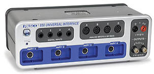
In the studio sessions, you will also collect data using Pasco 850 interface and the Capstone software.
The Pasco 850 interface is a data acquisition system connected to the
computer. It can collect information from various analog and digital
sensors, and generate seven different output signals. This exercise will
familiarize you with this data acquisition system.
The instrument you will use today is the Pasco Wireless Smart Cart. The
Smart Cart is a cart equipped with a position decoder. Encoder wheel
measure how far it has moved. You will measure the
position of the Smart Cart on an inclined plane as a function of time.
Set up a track with one end elevated, by placing it on a thick book.
Watch the video
"Getting started with
the Pasco software", and use your experimental setup to perform the same
experiments. To lift the track, use a second book. Pause the video when needed, so that you can follow the procedure step by step
and learn about the capabilities of the data acquisition system.
Experiment Deliverables: (to be included in the your journal)
Visuals: your final graph in Capstone. Click Edit, Copy,
and then paste it into your journal. Do not copy the graph of another group.
The graphs of different groups will not look exactly the same, since the
books and launch speeds are different.
Analysis:
Do you think you are now familiar enough to acquire data using the Pasco
software? Please comment.
Convert your journal into a lab report.
Name: E-mail address:
Laboratory 1 Report
Make sure you completed the entire lab and answered all parts. Make
sure you show your work and inserted and properly labeled relevant tables
and plots in your journal.
Add a summary reflection at the end of your report in a short essay format.
Save your Word document (your name_lab1.docx), go to Canvas, Assignments, Lab
1, and submit your document.
 In the studio sessions, you will also collect data using Pasco 850 interface and the Capstone software.
The Pasco 850 interface is a data acquisition system connected to the
computer. It can collect information from various analog and digital
sensors, and generate seven different output signals. This exercise will
familiarize you with this data acquisition system.
In the studio sessions, you will also collect data using Pasco 850 interface and the Capstone software.
The Pasco 850 interface is a data acquisition system connected to the
computer. It can collect information from various analog and digital
sensors, and generate seven different output signals. This exercise will
familiarize you with this data acquisition system.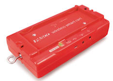 The instrument you will use today is the Pasco Wireless Smart Cart. The
Smart Cart is a cart equipped with a position decoder. Encoder wheel
measure how far it has moved. You will measure the
position of the Smart Cart on an inclined plane as a function of time.
The instrument you will use today is the Pasco Wireless Smart Cart. The
Smart Cart is a cart equipped with a position decoder. Encoder wheel
measure how far it has moved. You will measure the
position of the Smart Cart on an inclined plane as a function of time.