Free-fall - The acceleration of gravity

Gravity is the force of nature we are most aware of.  One can argue that other forces, such as the electromagnetic force, which holds molecules together in solid objects, or nuclear forces, which determine the structure of atoms, are more important, but these forces are less obvious to us.  Near the surface of Earth the force of gravity on an object of mass m equals F_g = mg.  It is constant and points straight down.  If we can neglect other forces and the net force is approximately equal to F_g, then we have motion with constant acceleration g.

Observation

Hold a tennis ball at about your height and then let go.  Observe the motion of the ball.

Describe the motion as the ball is falling.

• Estimate how long it takes the ball to reach the floor.
• What can you say about the speed of the ball as a function of the distance it has already fallen?
• If you drop the ball from about half of your height, does it take approximately half the time to reach the floor?

Experiment 1:  Tracking a freely falling object

It does not take the ball a long time to reach the floor.  It is hard to get detailed information about its motion without using external measuring instruments.  In this experiment, the instrument is a video camera.  You will analyze a video clip.  The clip shows a ball being dropped.  You will determine the position of the freely-falling ball as a function of time by stepping through the video clip frame-by-frame and by reading the time and the position coordinates of the ball off each frame.  You will construct a spreadsheet with columns for time and position and use this spreadsheet to find the velocity as a function of time.  The slope of a velocity versus time graph yields the acceleration of the ball.

Procedure:

To play the video clip or to step through it frame-by-frame click the "Begin" button.

• "Play" the video clip. When finished, "Step up" to frame 1.  In some browsers you have to click "Pause" first.
• In the setup window, choose to track the y-coordinate of an object.
• Click "Calibrate".  Then click "Calibrate Y".
  The video clip contains a meter stick.  Position the cursor over bottom end of the stick and click the left mouse button.  Then position the cursor over the top end of the stick and click the left mouse button again.   This will record the y-coordinates of the chosen positions.  Enter the distance between those positions into the text box in units of meter.  For the example positions, you would enter 1 into the text box.  Click "Done".
  Make sure the video frame stays fixed in the browser window between the two clicks.  You may have to scroll after the clicks to get to the buttons.
• Click the button "Click when done calibrating".  A spreadsheet will open up.  Click "Start taking data".
• Start tracking the ball.  Position the cursor over the ball.  When you click the left mouse button, the time and the y-coordinate of the ball will be entered into the spreadsheet.  You will automatically step to the next frame of the video clip.  Make sure the video frame stays fixed in the browser window while you take data.
• Repeat for each frame in the video clip until the ball reaches the bottom end of the meter stick.  Then click "Stop Taking Data".
  Highlight and copy your table.  Open Microsoft Excel, and paste the table into an Excel spreadsheet.  Depending on your browser, you may have to use "Paste" (Edge) or "Paste Special, Unicode Text" (Chrome).  Your spreadsheet will have two columns, time (s) and y (m).  If you followed the instructions above, the the y-axis points up.

Produce a graph of position versus time.  Label the axes.

• Describe your graph.  Does it resemble a straight line?  If not, what does it look like?
• Was the ball moving with constant velocity?  How can you tell?

For motion with constant acceleration we expect that y changes as a function of time as y = y₀ + v₀t + ½at², where a is the acceleration. For an object accelerating at a constant rate g we have y = y₀ + v₀t + ½gt², so y as a function of t is a polynomial of order 2 (a section of a parabola).  We can reduce numerical errors in finding the acceleration of the ball by fitting our position versus time data directly with a polynomial of order 2.

• Right-click the data in your position versus time graph and choose "Add Trendline".   Choose Polynomial, Order 2 and under options click "Display equation on chart".  An equation of the form y = b₁x² + b₂ x + b₃ will be displayed where b₁, b₂, and b₃ are numbers.  Since we are plotting y versus t, the number b₁ is the best estimate for g/2 from the fit.  Therefore the value of the acceleration determined from the fit is g = 2b₁.  Since our y-axis points upward, we expect a to be close to g = -9.8 m/s².
 
• Does the polynomial of order 2 fit the data well?  What value do you obtain for the acceleration of the ball from this fit?

After collecting your time and position data, provide your table of data to an AI with this prompt: 'I have table with columns "time" and "y-position" for a falling ball. Write a Python script using Matplotlib to calculate velocity, plot y vs y and y vs y, and find the acceleration using a linear fit on the velocity data.'  Run this code in Google Colab.  How does the AI's acceleration value compare to your Excel trendline?  Which method was more prone to error?

Experiment 1 Deliverables: (to be included in the your journal)

• Visuals:  Labeled plot of position versus time (Excel, including trendline) and of velocity versus time (AI generated).

• Analysis:  Compare the two fits.  Do they produce the same value for the acceleration?  How do these values compare to the accepted value for g.  What are some possible sources of error?

• Outcome:  The value(s) you obtain from the fits for the acceleration of the ball. 

Projectile motion

Experiment 2:  Tracking an object moving in two dimensions

A ball is moving in two dimensions under the influence of a constant gravitational force.  It is hard to get detailed information about its motion without using external measuring instruments.  In this experiment, the instrument is a video camera.  You will analyze a video clip.  The clip shows a ball being thrown.  You will determine the position of the ball in two dimensions as a function of time by stepping through the video clip frame-by-frame and by reading the time and the position coordinates of the ball off each frame.  You will construct a spreadsheet with columns for time and position and use this spreadsheet to find the x and y component of the velocity as a function of time.

Procedure:

To play the video clip or to step through it frame-by-frame click the "Begin" button.

• "Play" the video clip. When finished, "Step up" to frame 1.
• In the setup window, choose to track both coordinate of the object.
• Click "Calibrate". 
• Click "Calibrate X". 
  The video clip contains two meter sticks.  Position the cursor over left end of the horizontal stick and click the left mouse button.  Then position the cursor over the right end of the horizontal stick and click the left mouse button again.   This will record the x-coordinates of the chosen positions.  Enter the distance between those positions into the text box in units of meter.  For the example positions, you would enter 1 into the text box.  Click "Done".
  Make sure the video frame stays fixed in the browser window between the two clicks.  You may have to scroll after the clicks to get to the buttons.
• Now click "Calibrate Y".
  Position the cursor over bottom end of the vertical stick and click the left mouse button.  Then position the cursor over the top end of the vertical stick and click the left mouse button again.   This will record the y-coordinates of the chosen positions.  Enter the distance between those positions into the text box in units of meter.  For the example positions, you would enter 1 into the text box.  Click "Done".
  Make sure the video frame stays fixed in the browser window between the two clicks.
• Click the button "Click when done calibrating".  A spreadsheet will open up.  Click "Start taking data".
• Start tracking the ball.  Position the cursor over the ball.  When you click the left mouse button, the time and the x- and y-coordinates of the ball will be entered into the spreadsheet.  You will automatically step to the next frame of the video clip.  Make sure the video frame stays fixed in the browser window while you take data.  When the ball is caught, click "Stop Taking Data".
• Your table will have 3 columns, time (s), x( m), and y (m).
• Open Microsoft Excel, and paste the table into an Excel spreadsheet.

Produce graphs of the x and y components of position versus time.  Label the axes.

• Describe the graphs.  Does one of the graphs resemble a straight line?  If yes, what does this tell you?
• Right-click your data in the x(m) versus time graph and choose "Add Trendline".  Choose "Type, Linear" and "Options, Display equation on chart".  An equation y = ax + b will appear on your graph, where the number a is the slope and the number b is the y-intercept.  What is the physical meaning of the slope of this graph?
• Right-click the data in your y(m) versus time graph and choose "Add Trendline".  Choose Polynomial, Order 2 and under options click "Display equation on chart".  An equation of the form y = b₁x² + b₂ x + b₃ will be displayed where b₁, b₂, and b₃ are numbers.  What do the coefficients b₁ and b₂ tell you?
 
• We can view the motion of a projectile as a superposition of two independent motions.  Describe those two motions.

Experiment 2 Deliverables: (to be included in the your journal)

• Visuals:  Labeled plots (including trendline) of  x and y components of position versus time.

• Analysis:  What do the plots of the x and y components of position versus time tell you about the motion of the ball?

• Outcome:  Your experimental value of the horizontal component of the elocity and the vertical component of the acceleration.

Experiment 3:  Measuring the coefficient of static and kinetic friction

In this session you will measure the coefficient of static friction for a wood block and a felt-covered block in contact with a metal track.  The surface of the track makes an angle θ with the horizontal.  For angles θ > θ_max the block will accelerate down the sloping track.

You will determine the angle θ_max for which the maximum force of static friction f_{s_max} = μ_sN = μ_smg cosθ_max just cancels the component of the gravitational force f_g = mg sinθ_max pointing down the track.  You will then solve for the coefficient of static friction μ_s.

You have a track, a wood block, a scale, and two rulers.

• Determine the mass of the block using the electronic balance
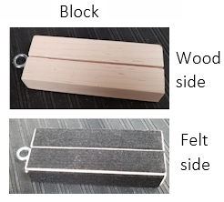
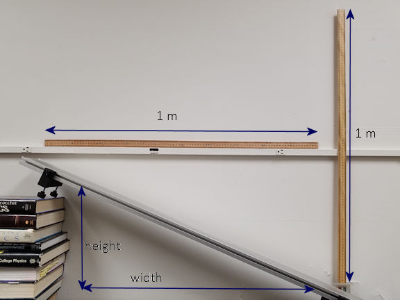
• Place the block on the track, with either the wood or the felt side touching the track.  Slowly increase the angle the track makes with the horizontal.  Measure the angle the track makes with the horizontal at which the block starts to accelerate.  Use the rulers to measure the width and height of a triangle and use tanθ = height/width.  You can also use an app on your phone to measure the angle.  I recommend that you install the app PhyPhox on your smartphone (iPhone or Andoid).  It gives you access to most of the sensors in your phone and has setups for many experiments. 
• Determine μ_s for the wood block and the felt-covered block.
  Construct a table as shown below.
   

  surface	θmax (deg)	μs
  wood
  felt

Measure μ_s for the wood block and the felt-covered block using a different method.

• Put the block on the horizontal track on the table, with either the wood or the felt side touching the track.
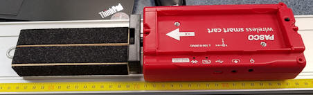
• Turn on your Smart Cart with the magnetic bumper attached to the force-sensor side.  In Capstone, add it to your devices under Hardware Setup.  Choose to measure Force (N).
• Create a Graph Display by dragging the Graph icon onto the main display.  Select Force, (N) for the y-axis and time (s) for the x-axis.
• Zero the force sensors.
• Start taking data.
  
• Gently push the cart with the bumper side against the block.  Increase the force until the block starts to move and then move it very slowly for a short amount of time.  Repeat a few times.  Make sure the force sensor reads zero when you are not pushing.

• What is the maximum force you have to apply to the block, with  the wood side touching the track, to start it moving?
  What is the maximum force you have to apply to the block, with  the felt side touching the track, to start it moving?
• f_{s_max}/N = f_{s_max}/(mg) = μ_s.  What values do you obtain from this experiment for the coefficient of static friction μ_s for a wood block and a felt-covered block in contact with a metal track?

Experiment 3 Deliverables: (to be included in the your journal)

• Analysis:  Explain how you measured the angle θ_max.  Comment on your results.  Compare the values μ_s obtained from the two measurements.  Are they close?  Are they very different?  Should they be the same?
  Describe your experimental setup to an AI.  Prompt: 'I measured a static friction coefficient of [your value] for wood on metal.  What environmental factors (humidity, surface roughness, track material) could explain why this differs from the standard value of 0.4?'  Incorporate the AI's insights into your analysis.

• Outcome:  Table of  θ_max and μ_s for wood and felt.

Convert your journal into a lab report.

Name:
E-mail address:

Laboratory 3 Report

• Make sure you completed the entire lab and answered all parts.  Make sure you show your work and inserted and properly labeled relevant tables and plots in your journal.
• Add a summary reflection at the end of your report in a short essay format.

Save your Word document (your name_lab3.docx), go to Canvas, Assignments, Lab 3, and submit your document.